The intelligentF1 Model

In each Formula One race there are over 1000 laps run (barring significant misfortunes), which provides a huge amount of data to be analysed. The intelligentF1 model provides the means of analysis uncovering trends of underlying pace and details of car performance which are not immediately obvious, and rarely commented upon especially if it is something that the teams would rather not tell you about.

The model has a number of elements; fuel load, tyre type and age, tyre degradation with a phase 2 accelerated degradation model, pitstop time loss and a methodology to handle safety car deployment. When the models for these elements are correct, the races of the cars in clear air can be simulated  – exactly as is done by the strategy guys at the teams (except that they have much, much more data) – and the strategy permutations which show which cars are really racing each other can be understood.

So what data is simulated?

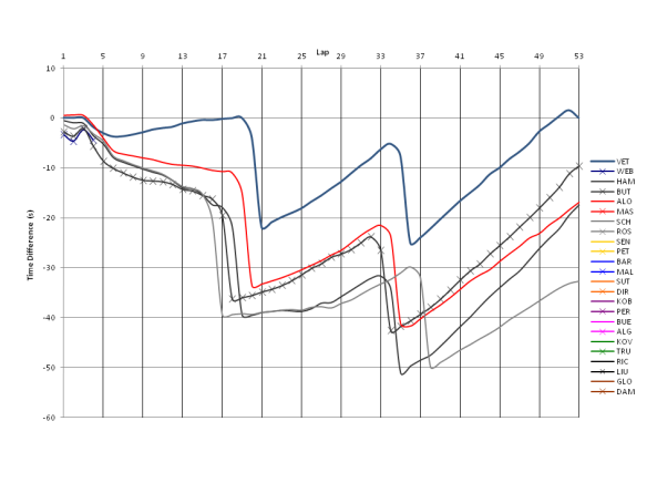
As the laptime data comes in during the race, the intelligentF1 model builds a Race History Chart with all the cars’ data. This can be manipulated to follow a given car over a given set of laps. An example Race History Chart is shown below for the first five cars in the 2011 Italian Grand Prix.

The horizontal axis is lap number, and the vertical axis shows the time each car is in front of (or behind) a reference average race time. This reference average time is often taken as the race time for the winner, such that the line representing the winner finishes at zero as it does for Vettel in the chart above. As this reference time is arbitrary, it can be set to different values to best view the race performances of different cars – this has the effect of shifting the lines up and down the graph.

The performance of each car can be seen in the lines running from left to right. The key for all cars is on the right. So we can see Vettel pulling away at the front, Schumacher and Hamilton battling and Button passing them at the end of the first stint and then passing Alonso in the final stint. The sudden drops in the lines are due to the time lost in pitstops. Up to this point, this is the same as the data which can be found in other places, such as FORIX.

How is the data simulated?

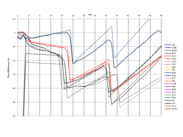
Now we have this data, we can simulate the races using the intelligentF1 model. The same Race History Chart is shown below with the addition of the dashed lines showing the intelligentF1 model simulation of the race.

The pace of each car is determined by the gradient of the line, the faster the car, the steeper the gradient. The intelligentF1 model matches the gradient of the line in a stint where the car is in clear air (not always available) and can then predict the pace of the cars at other stages of the race. As can be seen, some gradients match and others don’t.

So how do you know it’s right?

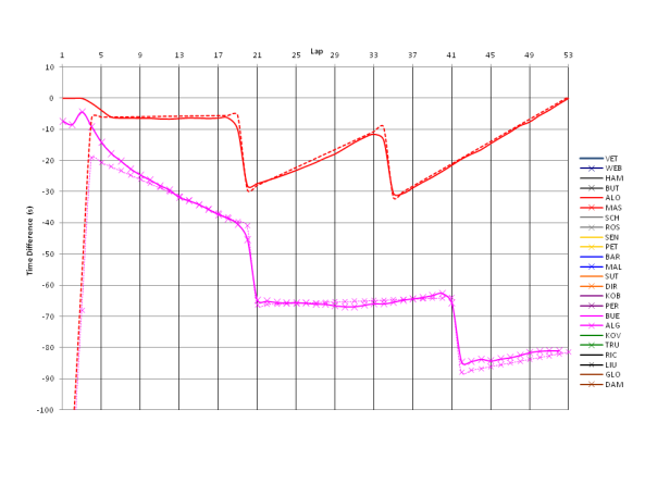
There is a big difference between being right, and being good enough to understand the data and what it really means. There will be variations in a driver’s performance from lap to lap and mistakes, spins, overtaking manoeuvres, pitstop errors and times when a car is trapped behind a slower car. None of this can be predicted. However, these are the best cars and drivers in the world, and this means that there is actually a high level of consistency in their performance (outside these occasional unpredictable events), and this is usually at a level very close to their optimum. Therefore, when a car is in clear air, the intelligentF1 model is able to infer the underlying pace of the car/driver combination, and extrapolate this to other stages of the race. Consistency across a race, or stints from a number of drivers provides validation of the fuel and tyre models. For example, consider the simulations of the races of Alonso and Alguersuari at the 2011 Italian Grand Prix in the chart below. The intelligentF1 model simulations are very good showing that the models prediction of underlying pace is accurate enough to start doing more interesting things.

What can it tell you?

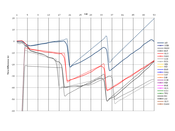
Where the intelligentF1 model is powerful is in allowing assessment of the data where things are not so simple and the traces do not match the predictions.  Let’s take some examples from the 2011 Italian Grand Prix at Monza, as this was a nice straightforward two-stop race. Firstly, let’s look at the races of Vettel, Schumacher and Hamilton. I have also put Alonso’s trace on the figure below.

The intelligentF1 model matches Vettel’s first stint, but then suggests he should be going about 0.5s faster in the remaining stints. So either Seb was so seriously underfuelled for the race and needed to back off for two-thirds of the race (which would be a horrible mistake), or he was cruising, matching his pace to the fastest cars behind – the McLarens. The intelligentF1 model suggests here that he could have won by 30s if he’d wanted. Could Hamilton have beaten him if he had got to the first corner first? This pace advantage suggests it would be very unlikely.

Now let’s look at Schumacher’s trace. His pace is nice and consistent for much of the first stint, until Hamilton really starts pressing, and he starts struggling with his tyres. The second stint is where it gets interesting. Michael’s pace is much slower due to the pressure from Lewis, and is quite inconsistent. However, once Lewis goes past, Michael’s pace then increases beyond what would be expected from the first stint. The most likely explanation for this is that in going slower he was stressing his tyres less, and then had more tyre life left at the end of the stint than would be expected. Mercedes then let him go for as long as he could maintain this pace, resulting in a longer stint and the recovery of most of the time lost in battling Lewis. He loses a bit in the final lap before his pitstop, though.

Once past, Hamilton was able to use his pace to open a gap, to stay ahead at the final stops and to start chasing down the Ferrari ahead of him. However, by looking at the first couple of laps after his stop, it is clear that he was not chasing as hard as he might have been until alerted to the possibilties by a radio call from the team. The intelligentF1 model projects that had he used his full pace, he would have caught Alonso with about three laps to go. An opportunity missed.

Where does it develop from here?

The intelligentF1 model will be applied to upcoming Formula One races to simulate the underlying pace of the cars and drivers, to analyse strategic decisions, and to paint a clearer picture of why the race turned out the way it did. Perhaps it can even be done in real time…